金桔
金币
威望
贡献
回帖0
精华
在线时间 小时
|
登陆有奖并可浏览互动!
您需要 登录 才可以下载或查看,没有账号?立即注册


×
本人已委托维权骑士(http://www.rightknights.com)进行原创维权。
思想高屋建瓴,知识原创共享。
转载请引用链接。
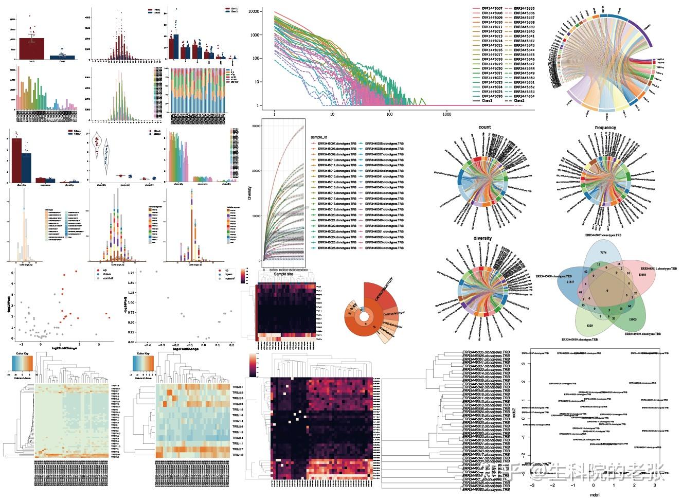
<hr/>免疫组库(Immune Repertoire,IR)是指某个个体在任何特定时间点其循环系统中所有功能多样性B淋巴细胞和T淋巴细胞的总和。免疫组库分析是指通过高通量测序技术,对机体免疫组库的多样性及每种 T、B细胞克隆的独特性序列组成和变化进行分析,从而全面评估机体的免疫状态,明确疾病与T、B细胞克隆组成及变化之间的关系,是免疫学和医学领域常用的分析方法。
<hr/>1.1 MiXCR and VDJtools:
从 Releases · milaboratory/mixcr 和 Release 1.2.1 · mikessh/vdjtools下载MiXCR和VDJtools的压缩包并解压。
1.2 Java Runtime Environment (JRE, at least v1.8)
从 https://java.com/en/download/ 下载Java组件并按照提示安装,因为MiXCR和VDJtools都基于java编写,因此需要java运行。
1.3 R packages VDJtools needs:
VDJTools的可视化依赖于R的一些可视化包如我们使用过的circlize等,因此需要安装这些R包,清单如下:
- ape
- circlize
- FField
- ggplot2
- gplots
- grid
- gridExtra
- MASS
- plotrix
- RColorBrewer
- reshape
- reshape2
- scales
- VennDiagram
可在R中手动安装,也可以在命令行通过以下代码安装:
java -jar /path/to/vdjtools/vdjtools.jar Rinstall
#/path/to/vdjtools/为vdjtools.jar的所在路径1.4 免疫组库数据:
一方面,从理论上来说,只要测序覆盖了T细胞CDR或B细胞IG的编码区,就可以从测序数据中提取出免疫组信息。另一方面,根据MiXCR官网的描述,除了靶向建库的免疫组库测序数据,也可以使用RNA-Seq或其他非靶向但覆盖有免疫组信息的测序数据作为输入。
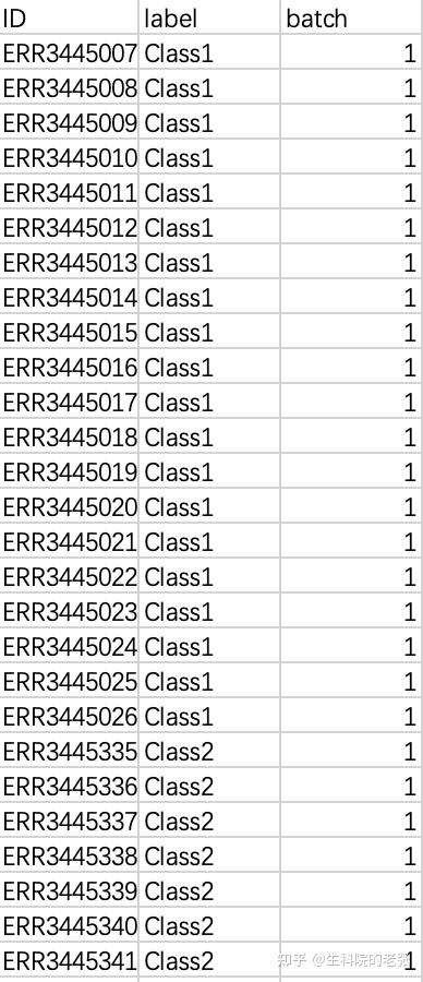
1.5 免疫组库数据对应的样本信息:
包含有所有样本的分组信息,以便后续的分组分析,文件格式参考如下:
<hr/>2. 分析流程:
2.1 通过fastqc、multiqc、trimmomatic进行质量过滤:
和其他基因测序数据一样,拿到数据后首先要通过fastqc、multiqc、trimmomatic进行质量过滤,详细步骤可见我之前的文章 生科院的老张:RNAseq转录组差异表达分析教程 .
2.1.1 md5检查数据完整性:
md5sum *gz > md5.txt && md5sum -c md5.txt
# *gz 任意以gz结尾的文件
# > 运行结果保存至
# && 连接符,前一命令完成继续执行下一命令2.1.2 fastqc质量控制与multiqc合并质控报告:
fastqc *gz && multiqc ./
# 对所有gz结尾文件进行质控并对当前目录下所有质控报告进行合并2.1.3 trimmomatic质量过滤:
trimmomatic
PE #双端测序,单端测序为SE
-threads 4 #指定线程数为4
~/WES_WGS_WGRS/data/sample1/sample1_1.fq.gz #输入序列
~/WES_WGS_WGRS/data/sample1/sample1_2.fq.gz
~/WES_WGS_WGRS/data/sample1/sample1_paired_clean_1.fq.gz #输出配对序列和非配对序列
~/WES_WGS_WGRS/data/sample1/sample1_unpair_clean_1.fq.gz
~/WES_WGS_WGRS/data/sample1/sample1_paired_clean_2.fq.gz
~/WES_WGS_WGRS/data/sample1/sample1_unpair_clean_2.fq.gz
ILLUMINACLIP:/data1/guest/yinlei/miniconda3/pkgs/trimmomatic-0.39-1/share/trimmomatic/adapters/TruSeq3-PE-2.fa:2:30:10:1:true
#去除ILLUMINA接头,根据质控报告选择trimmomatic文件夹adapters路径下的接头文件
LEADING:3 #从reads开头切除质量低于阈值3的碱基
TRAILING:3 #从reads末尾切除质量低于阈值3的碱基
SLIDINGWINDOW:4:20 #从reads 5‘端开始进行长度为4的滑窗过滤,切除碱基质量低于阈值20的碱基
MINLEN:50 #丢弃剪切后长度低于阈值50的reads
TOPHRED33 #将reads的碱基质量值体系转为phred-33,若为phred-64则为TOPHRED64<hr/>2.2 MiXCR提取免疫组信息:
#for targeted TCR/IG libraries
java -jar /path/to/mixcr/mixcr.jar
analyze amplicon
-s hsa --starting-material dna --5-end v-primers --3-end j-primers --adapters adapters-present
sample1_1.fastq sample1_2.fastq /path/mixcr_result/sample1
#for non-enriched data
java -jar /path/to/mixcr/mixcr.jar
analyze shotgun
-s hsa --starting-material dna
sample1_1.fastq sample1_2.fastq /path/mixcr_result/sample1以下为结果文件:
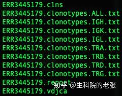
MiXCR结果文件
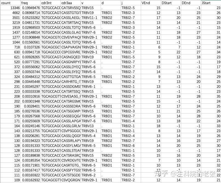
包含了IG和CDR的信息,本文以TCR betta 链的分析为例,如下为TRB文件的格式:
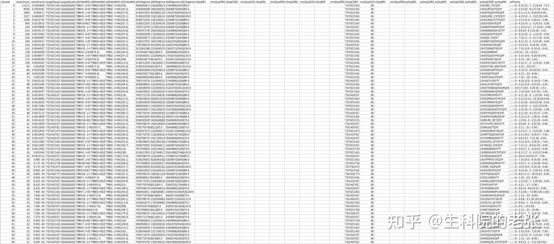
.clonotypes.TRB.txt文件格式
包含有clonotype,氨基酸序列,核苷酸序列,reads计数,V(D)J基因组成等信息。
<hr/>2.3 格式转换:
将MiXCR输出格式转换为VDJtools支持的输入格式,通过以下代码实现:
java -jar /path/to/vdjtools/vdjtools-1.2.1.jar
Convert -S mixcr path/to/mixcr_result/*.TRB.txt /path/to/vdjtools_result/输出文件格式如下:
<hr/>2.4 基础分析:
对格式转换后的文件进行后续分析。
java -jar /path/to/vdjtools/vdjtools-1.2.1.jar
CalcBasicStats sample1.txt sample2.txt sample3.txt... /path/to/vdjtools_result/输出文件包含有各样本的基础信息,格式如下:
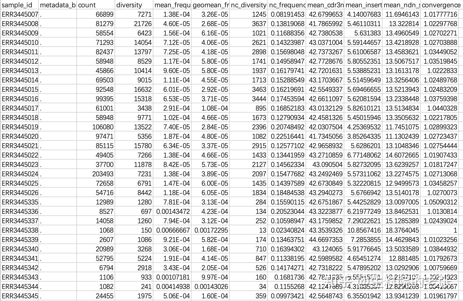
<hr/>2.5 CDR3 Clonotypes Richness:
import seaborn as sns, matplotlib.pyplot as plt
########################################################################################################################
input_path='/Users/ZYP/Downloads/imm_repertoire/vdjtools_result/'#输入路径
output_path='/Users/ZYP/Downloads/imm_repertoire/vdjtools_result/'#输出路径
sample_info='sample_info.txt'#记录有样本分组的样本信息
########################################################################################################################
list_pos=[]
for line in open(input_path+sample_info,'r'):
info=line[:-1].split('\t')
if info[0]!='ID':
if str(info[1])=='Class1':
list_pos.append(info[0])
list_class=[]
list_sample=[]
list_richness=[]
for line in open(output_path+'basicstats.txt','r'):
info=line[:-1].split('\t')
if info[0]!='sample_id':
if info[0].split('.')[0] in list_pos:
list_class.append('Class1')
else:
list_class.append('Class2')
list_sample.append(info[0].split('.')[0])
list_richness.append(float(info[3]))
ax1 = sns.barplot(x=list_class,y=list_richness,capsize=.2,palette=(sns.xkcd_rgb["dark red"],sns.xkcd_rgb["marine blue"]))
ax1_1 = sns.stripplot(x=list_class,y=list_richness,size=5,palette=(sns.xkcd_rgb["dark red"],sns.xkcd_rgb["marine blue"]))
ax1.spines['top'].set_visible(False)
ax1.spines['right'].set_visible(False)
plt.savefig(output_path+'Richness_barplot_Class.pdf')
plt.show()
ax2 = sns.barplot(x=list_sample,y=list_richness)
ax2.set_xticklabels(ax2.get_xticklabels(), rotation=-90)
ax2.spines['top'].set_visible(False)
ax2.spines['right'].set_visible(False)
plt.savefig(output_path+'Richness_barplot_Sample.pdf')
plt.show()结果如下图所示:
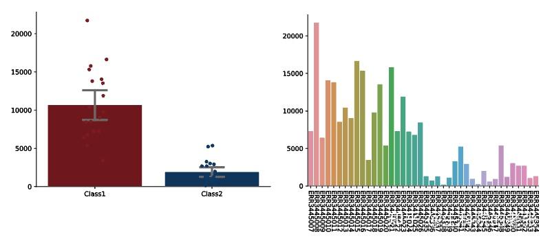
CDR3 Clonotypes Richness
<hr/>2.6 CDR3 Clonotypes Length:
import seaborn as sns, matplotlib.pyplot as plt
########################################################################################################################
input_path='/Users/ZYP/Downloads/imm_repertoire/vdjtools_input/'#输入路径
output_path='/Users/ZYP/Downloads/imm_repertoire/vdjtools_result/'#输出路径
sample_info='sample_info.txt'#记录有样本分组的样本信息
########################################################################################################################
dict_sample_LengthCount={}
list_pos=[]
for line in open(input_path+sample_info,'r'):
info=line[:-1].split('\t')
id=info[0]
if id!='ID':
if str(info[1])=='Class1':
list_pos.append(id)
read_file=open(input_path+id+'.clonotypes.TRB.txt','r')
dict_length_count={}
for line in read_file:
if line[0]!='c':
length=len(line[:-1].split('\t')[3])
if length < 30:
if length not in dict_length_count.keys():
dict_length_count[length]=1
else:
dict_length_count[length]+=1
dict_sample_LengthCount[id]=dict_length_count
read_file.close()
list_length=[]
list_class=[]
list_sample=[]
list_count=[]
for sample in dict_sample_LengthCount.keys():
dict_length_count=dict_sample_LengthCount[sample]
for length in dict_length_count.keys():
list_length.append(length)
list_sample.append(sample)
if sample in list_pos:
list_class.append('Class1')
else:
list_class.append('Class2')
list_count.append(dict_length_count[length])
ax1 = sns.barplot(x=list_length,y=list_count,hue=list_class,errwidth=0.5,capsize=0.5,palette=(sns.xkcd_rgb["dark red"],sns.xkcd_rgb["marine blue"]))
ax1_1 = sns.stripplot(x=list_length,y=list_count,hue=list_class,size=2,dodge=True,palette=(sns.xkcd_rgb["dark red"],sns.xkcd_rgb["marine blue"]))
ax1.set_xticklabels(ax1.get_xticklabels(), rotation=-90,fontsize=6)
ax1.spines['top'].set_visible(False)
ax1.spines['right'].set_visible(False)
plt.savefig(output_path+'Length_barplot_Class.pdf')
plt.show()
ax2 = sns.barplot(x=list_length,y=list_count,hue=list_sample,errwidth=0.5,capsize=0.5)
ax2.set_xticklabels(ax2.get_xticklabels(), rotation=-90,fontsize=6)
ax2.spines['top'].set_visible(False)
ax2.spines['right'].set_visible(False)
plt.savefig(output_path+'Length_barplot_Sample.pdf')
plt.show()结果如下图所示:
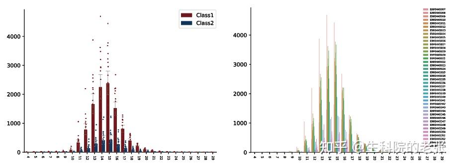
CDR3 Clonotypes Length
<hr/>2.7 CDR3 Clonotypes Abundance Proportion:
import numpy as np, seaborn as sns, matplotlib.pyplot as plt
########################################################################################################################
input_path='/Users/ZYP/Downloads/imm_repertoire/vdjtools_input/'#输入路径
output_path='/Users/ZYP/Downloads/imm_repertoire/vdjtools_result/'输出路径
sample_info='sample_info.txt'#记录有样本分组的样本信息
########################################################################################################################
dict_sample_ReadsCounts={}
list_pos=[]
for line in open(input_path+sample_info,'r'):
info = line[:-1].split('\t')
id = info[0]
if id != 'ID':
if str(info[1]) == 'Class1':
list_pos.append(id)
read_file = open(input_path + id + '.clonotypes.TRB.txt', 'r')
dict_read_count={'1':0,'2-3':0,'4-10':0,'11-30':0,'31-100':0,'101-MAX':0}
number_clonotypes=0
for line in read_file:
if line[0] != 'c':
number_clonotypes+=1
info=line[:-1].split('\t')
count=info[0]
if int(count) == 1:
dict_read_count['1']+=1
elif int(count) in [2,3]:
dict_read_count['2-3']+=1
elif 4 <= int(count) <= 10:
dict_read_count['4-10']+=1
elif 11 <= int(count) <= 30:
dict_read_count['11-30']+=1
elif 31 <= int(count) <= 100:
dict_read_count['31-100']+=1
elif int(count) >= 101:
dict_read_count['101-MAX']+=1
for key in dict_read_count:
dict_read_count[key]=dict_read_count[key]/number_clonotypes*100
dict_sample_ReadsCounts[id]=dict_read_count
read_file.close()
list_sample=[]
list_class=[]
list_read=[]
list_count=[]
dict_read_SampleCount={'1': {},'2-3': {},'4-10': {},'11-30': {},'31-100': {},'101-MAX': {}}
print(dict_sample_ReadsCounts)
for sample in dict_sample_ReadsCounts.keys():
dict_read_count=dict_sample_ReadsCounts[sample]
for read in dict_read_count.keys():
list_sample.append(sample)
if sample in list_pos:
list_class.append('Class1')
else:
list_class.append('Class2')
list_read.append(read)
count=float(dict_read_count[read])
list_count.append(count)
dict_sample_count=dict_read_SampleCount[read]
dict_sample_count[sample]=count
dict_read_SampleCount[read]=dict_sample_count
ax1 = sns.barplot(x=list_read,y=list_count,hue=list_class,errwidth=1,capsize=0.2,palette=(sns.xkcd_rgb["dark red"],sns.xkcd_rgb["marine blue"]))
ax1_1 = sns.stripplot(x=list_read,y=list_count,hue=list_class,dodge=True,palette=(sns.xkcd_rgb["dark red"],sns.xkcd_rgb["marine blue"]))
ax1.set_xticklabels(ax1.get_xticklabels(), rotation=-90,fontsize=6)
ax1.spines['top'].set_visible(False)
ax1.spines['right'].set_visible(False)
plt.savefig(output_path+'CountProportion_lappedplot_Class.pdf')
plt.show()
fig,ax = plt.subplots()
list_1=[]
list_2_3=[]
list_4_10=[]
list_11_30=[]
list_31_100=[]
list_101_MAX=[]
for read in dict_read_SampleCount.keys():
dict_sample_count=dict_read_SampleCount[read]
list_sample=[]
for sample in dict_sample_count.keys():
list_sample.append(sample)
if read=='1':
list_1.append(dict_sample_count[sample])
elif read=='2-3':
list_2_3.append(dict_sample_count[sample])
elif read=='4-10':
list_4_10.append(dict_sample_count[sample])
elif read=='11-30':
list_11_30.append(dict_sample_count[sample])
elif read=='31-100':
list_31_100.append(dict_sample_count[sample])
elif read=='101-MAX':
list_101_MAX.append(dict_sample_count[sample])
list_1=np.array(list_1)
list_2_3=np.array(list_2_3)
list_4_10=np.array(list_4_10)
list_11_30=np.array(list_11_30)
list_31_100=np.array(list_31_100)
list_101_MAX=np.array(list_101_MAX)
width = 0.35
print(list_1)
ax.bar(list_sample,list_1,width, label='1')
ax.bar(list_sample,list_2_3,width,label='2_3',bottom=list_1)
ax.bar(list_sample,list_4_10,width,label='4-10',bottom=list_1+list_2_3)
ax.bar(list_sample,list_11_30,width,label='11-30',bottom=list_1+list_2_3+list_4_10)
ax.bar(list_sample,list_31_100,width,label='31-100',bottom=list_1+list_2_3+list_4_10+list_11_30)
ax.bar(list_sample,list_101_MAX,width,label='101-MAX',bottom=list_1+list_2_3+list_4_10+list_11_30+list_31_100)
ax.spines['top'].set_visible(False)
ax.spines['right'].set_visible(False)
ax.legend()
ax.set_xticklabels(list_sample, rotation=90, fontsize=10)
plt.savefig(output_path+'CountProportion_barplot_sample.pdf')
plt.show()结果如下图所示:
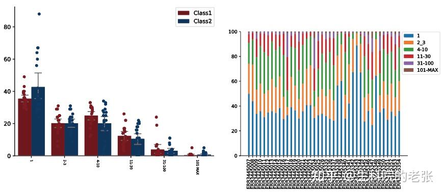
CDR3 Clonotypes Abundance Proportion:
<hr/>2.8 The relationship between CDR3 Abundance and CDR3 Clonotypes Richness:
import seaborn as sns, matplotlib.pyplot as plt
########################################################################################################################
input_path='/Users/ZYP/Downloads/imm_repertoire/vdjtools_input/'#输入路径
output_path='/Users/ZYP/Downloads/imm_repertoire/vdjtools_result/'输出路径
sample_info='sample_info.txt'#记录有样本分组的样本信息
########################################################################################################################
dict_sample_AbundanceRichness={}
list_pos=[]
for line in open(input_path+sample_info,'r'):
info = line[:-1].split('\t')
id = info[0]
if id != 'ID':
if str(info[1]) == 'Class1':
list_pos.append(id)
dict_abundance_richness={}
read_file = open(input_path + id + '.clonotypes.TRB.txt', 'r')
for line in read_file:
if line[0]!='c':
info=line[:-1].split('\t')
abundance=info[0]
if abundance not in dict_abundance_richness.keys():
dict_abundance_richness[abundance]=1
else:
dict_abundance_richness[abundance]+=1
dict_sample_AbundanceRichness[id]=dict_abundance_richness
read_file.close()
list_abundance=[]
list_richniess=[]
list_sample=[]
list_class=[]
for sample in dict_sample_AbundanceRichness.keys():
dict_abundance_richness=dict_sample_AbundanceRichness[sample]
for abundance in dict_abundance_richness.keys():
list_sample.append(sample)
if sample in list_pos:
list_class.append('Class1')
else:
list_class.append('Class2')
list_abundance.append(int(abundance))
list_richniess.append(int(dict_abundance_richness[abundance]))
ax = sns.lineplot(x=list_abundance,y=list_richniess,hue=list_sample,style=list_class)
ax.spines['top'].set_visible(False)
ax.spines['right'].set_visible(False)
plt.xscale('log')
plt.yscale('log')
plt.savefig(output_path+'Abundance_Proportion_relatplot.pdf')
plt.show()结果如下图所示:
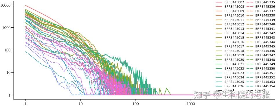
The relationship between CDR3 Abundance and CDR3 Clonotypes Richness
<hr/>2.9 CDR3 Overlap:
2.9.1 计算样本间CDR3重叠部分并写入本地文件overlapped_CDR3.txt:
########################################################################################################################
input_file=open('/Users/ZYP/Downloads/imm_repertoire/vdjtools_result/intersect.batch.aa.txt','r')#请将带有绝对路径的CalcPairwiseDistances的输出文件写在此处的''内
save_file=open('/Users/ZYP/Downloads/imm_repertoire/vdjtools_result/overlapped_CDR3.txt','w')#请将带有绝对路径的输出文件写在此处的''内
########################################################################################################################
list_samples=[]
diction={}
row=1
for line in input_file:
if row!=1:
info=line[:-1].split('\t')
for sample in [info[0],info[1]]:
if sample not in list_samples:
list_samples.append(sample)
key=info[0]+'and'+info[1]
value=info[4]
diction[key]=value
row+=1
input_file.close()
word=''
for sample in list_samples:
sample=sample.split('.')[0]
word+=sample+'\t'
save_file.write(word[:-1]+'\n')
for sample_row in list_samples:
word=''
for sample_column in list_samples:
if sample_row+'and'+sample_column in diction.keys():
word+=str(diction[sample_row+'and'+sample_column])+'\t'
else:
if sample_column+'and'+sample_row in diction.keys():
word+=str(diction[sample_column+'and'+sample_row])+'\t'
else:
word+='0'+'\t'
word=word[:-1]+'\n'
save_file.write(word)
save_file.close()2.9.2 CDR3 Overlap-heatmap:
import seaborn as sns, pandas as pd, matplotlib.pyplot as plt
########################################################################################################################
input_file='/Users/ZYP/Downloads/imm_repertoire/vdjtools_result/overlapped_CDR3.txt'#请将带有绝对路径的输入文件写在此处的''内
output_file='/Users/ZYP/Downloads/imm_repertoire/vdjtools_result/overlapped_CDR3.pdf'#请将带有绝对路径的输出文件写在此处的''内
########################################################################################################################
list_samples=[]
list_value_list=[]
number_row=1
for line in open(input_file):
if number_row!=1:
list_value=[]
index=0
for value in line[:-1].split('\t'):
list_value.append(float(value))
index+=1
list_value_list.append(list_value)
else:
for sample in line[:-1].split('\t'):
list_samples.append(sample)
number_row+=1
data=pd.DataFrame(data=list_value_list,index=list_samples,columns=list_samples)
ax=sns.clustermap(data,standard_scale=1,figsize=(19,19))
plt.savefig(output_file)
plt.show()结果如下图所示:
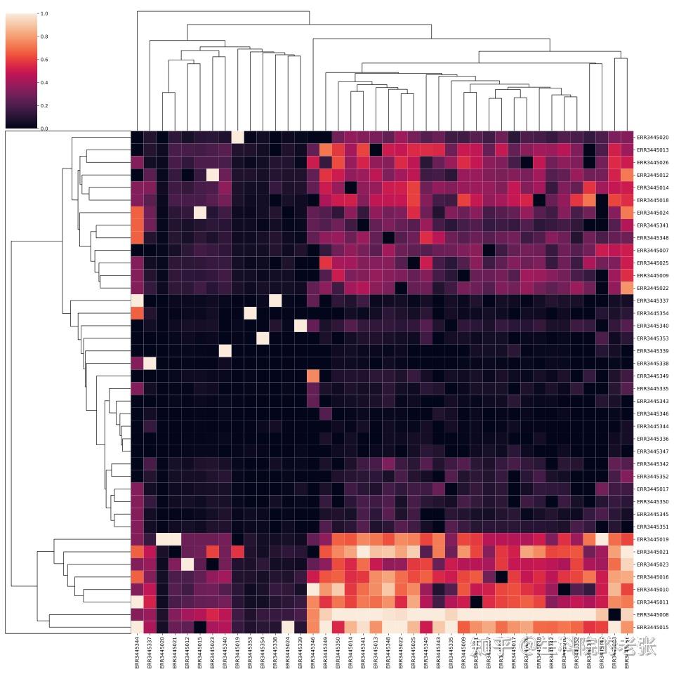
CDR3 Overlap-heatmap
2.9.3 CDR3 Overlap-circosplot-Vennplot:
#circosplot
java -jar /path/to/vdjtools/vdjtools.jar
CalcPairwiseDistances -p --low-mem
sample1.txt sample2.txt sample3.txt... ./vdjtools_result/
#vennplot
java -jar /path/to/vdjtools/vdjtools.jar
JoinSamples -p sample1.txt sample2.txt sample3.txt... ./vdjtools_result/结果如下图所示:
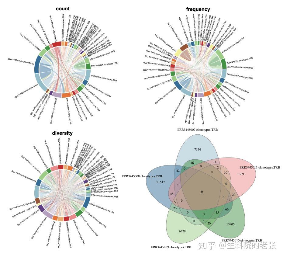
CDR3 Overlap-circosplot-Vennplot
<hr/>2.10 CDR3 diversity / evenness / clonality:
2.10.1 计算diversity / evenness / clonality 并可视化:
import math,seaborn as sns,matplotlib.pyplot as plt
########################################################################################################################
input_path='/Users/ZYP/Downloads/imm_repertoire/vdjtools_input/'#输入路径
output_path='/Users/ZYP/Downloads/imm_repertoire/vdjtools_result/'输出路径
sample_info='sample_info.txt'#记录有样本分组的样本信息
########################################################################################################################
def Shannon_entropy(list_frequency):
sum=0
for frequency in list_frequency:
sum+=frequency*math.log(frequency)
H=-sum
return H
def Pielou_evenness(H,richness):
E=H/math.log(richness)
return E
def Clonality(E):
C=1-E
return C
list_pos=[]
list_characteristic=[]
list_value=[]
list_sample=[]
list_class=[]
for line in open(input_path+sample_info,'r'):
info = line[:-1].split('\t')
id = info[0]
if id != 'ID':
if info[1] == 'Class1':
list_pos.append(id)
read_file = open(input_path + id + '.clonotypes.TRB.txt', 'r')
richness=0
TotalCount=0
for line in read_file:
if line[0] != 'c':
count = int(line[:-1].split('\t')[0])
richness+=1
TotalCount+=count
read_file.close()
read_file = open(input_path + id + '.clonotypes.TRB.txt', 'r')
list_frequency = []
for line in read_file:
if line[0] != 'c':
count = int(line[:-1].split('\t')[0])
list_frequency.append(count/TotalCount)
diversity=Shannon_entropy(list_frequency)
evenness=Pielou_evenness(diversity,richness)
clonality=Clonality(evenness)
list_characteristic+=['diversity','evenness','clonality']
list_value+=[diversity,evenness,clonality]
for time in range(0,3):
list_sample.append(id)
if id in list_pos:
list_class.append('Class1')
else:
list_class.append('Class2')
read_file.close()
print(list_class)
ax1 = sns.barplot(x=list_characteristic,y=list_value,hue=list_class,errwidth=0.5,capsize=0.3,palette=(sns.xkcd_rgb["dark red"],sns.xkcd_rgb["marine blue"]))
ax1_1 = sns.stripplot(x=list_characteristic,y=list_value,size=2,hue=list_class,dodge=True,palette=(sns.xkcd_rgb["dark red"],sns.xkcd_rgb["marine blue"]))
ax1.spines['top'].set_visible(False)
ax1.spines['right'].set_visible(False)
plt.savefig(output_path+'diversity_evenness_clonality_barplot_class.pdf')
plt.show()
ax2 = sns.violinplot(x=list_characteristic,y=list_value,hue=list_class,palette=('white','white'))
ax2_1 = sns.stripplot(x=list_characteristic,y=list_value,size=4,hue=list_class,dodge=True,palette=(sns.xkcd_rgb["dark red"],sns.xkcd_rgb["marine blue"]))
ax2.spines['top'].set_visible(False)
ax2.spines['right'].set_visible(False)
plt.savefig(output_path+'diversity_evenness_clonality_violinplot_class.pdf')
plt.show()
ax3 = sns.barplot(x=list_characteristic,y=list_value,hue=list_sample,errwidth=0.5,capsize=0.5)
ax3.spines['top'].set_visible(False)
ax3.spines['right'].set_visible(False)
plt.savefig(output_path+'diversity_evenness_clonality_sample.pdf')
plt.show()结果如下图所示:
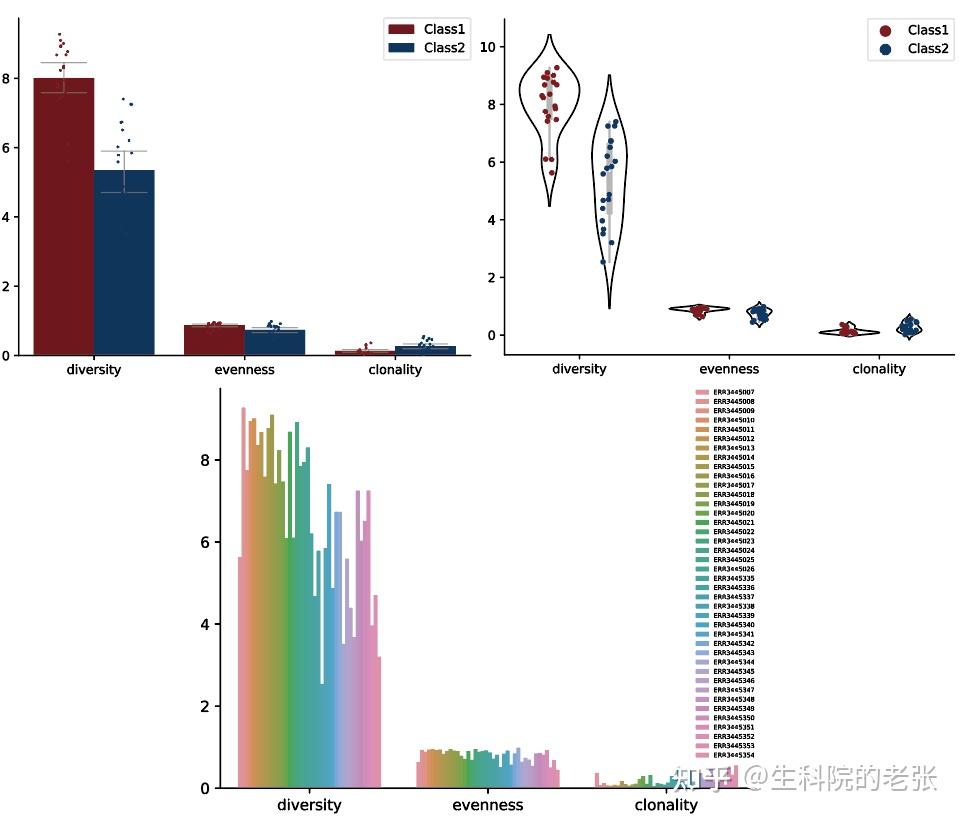
CDR3 diversity / evenness / clonality
2.10.2 The relationship between CDR3 Abundance and CDR3 diversity:
java -jar /path/to/vdjtools/vdjtools.jar
RarefactionPlot sample1.txt sample2.txt sample3.txt... ./vdjtools_result/结果如下图所示:
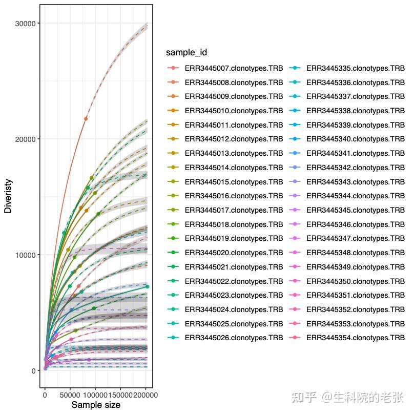
The relationship between CDR3 Abundance and CDR3 diversity
2.10.3 pieplot for 1 sample:
java -jar /path/to/vdjtools/vdjtools.jar
PlotQuantileStats -t 5 sample1.txt ./vdjtools_result/结果如下图所示:
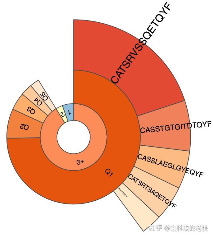
pieplot for 1 sample
<hr/>2.11 DR3 length distribution for 1 sample:
2.10.1 CDR3 length distribution among CDRs:
java -jar /path/to/vdjtools/vdjtools.jar
PlotFancySpectratype -t 20 sample1.txt /path/to/vdjtools_result/结果如下图所示:
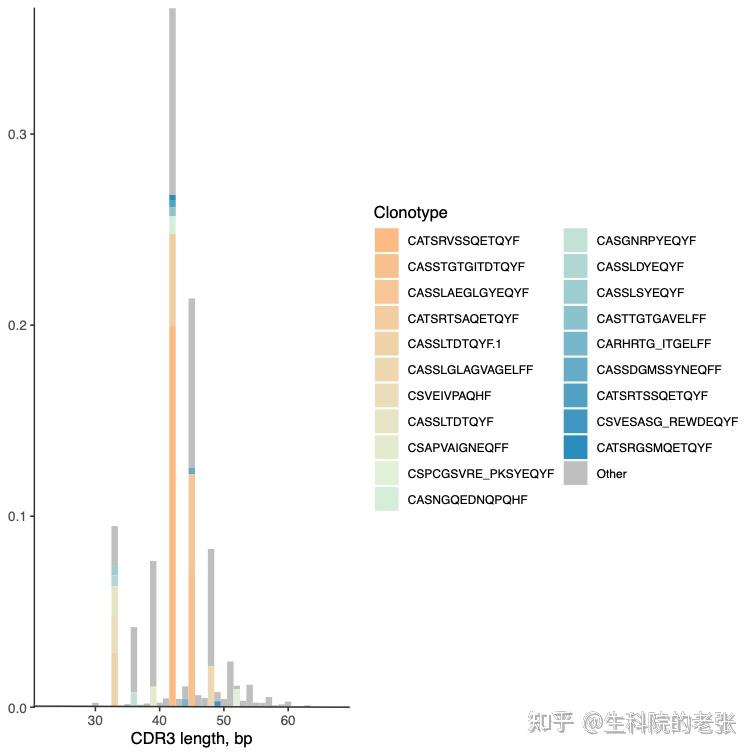
CDR3 length distribution among CDRs
2.11.2 CDR3 length distribution among genes based on clonotype / frequency:
#CDR3 length distribution based on clonotype number among Vgenes
java -jar /path/to/vdjtools/vdjtools.jar
PlotSpectratypeV -u sample1.txt /path/to/vdjtools_result/
#CDR3 length distribution based on read frequency among Vgenes
java -jar /path/to/vdjtools/vdjtools.jar
PlotSpectratypeV sample1.txt /path/to/vdjtools_result/结果如下图所示:
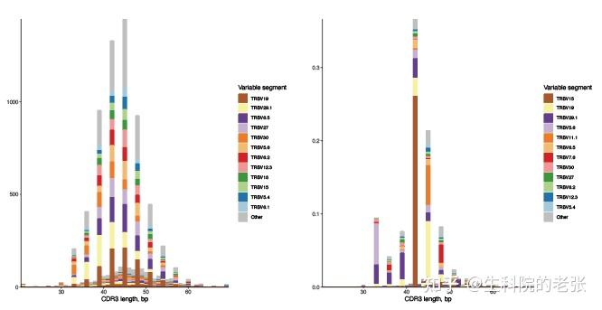
CDR3 length distribution among genes based on clonotype / frequency
<hr/>2.12 sample similarity based on CDR3:
java -jar /path/to/vdjtools/vdjtools.jar
ClusterSamples -p -l /path/to/vdjtools_result/ /path/to/vdjtools_result/结果如下图所示:
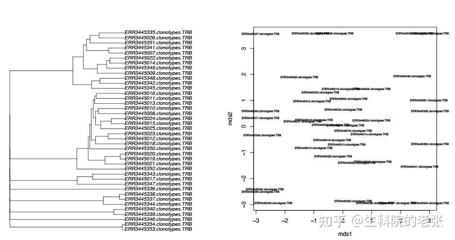
sample similarity based on CDR3
<hr/>2.13 gene usage:
java -jar /path/to/vdjtools/vdjtools.jar
CalcSegmentUsage -p sample1.txt sample2.txt sample3.txt... /path/to/vdjtools_result/结果如下图所示:
gene usage
<hr/>2.14 gene pairing for 1 sample:
java -jar /path/to/vdjtools/vdjtools.jar
PlotFancyVJUsage sample1.txt /path/to/vdjtools_result/结果如下图所示:
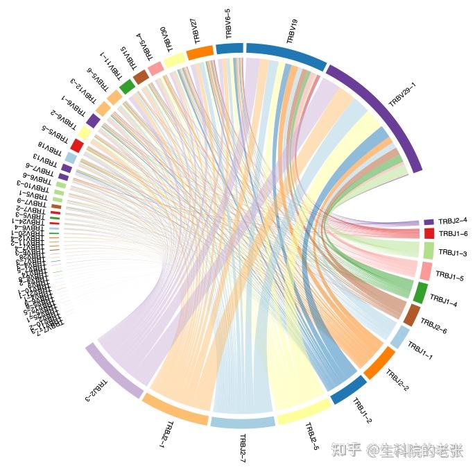
gene pairing for 1 sample
<hr/>2.15 gene diff-expression:
2.15.1 计算样本基因数:
path='/Users/ZYP/Downloads/imm_repertoire/'
sample_info=open(path+'vdjtools_result/sample_info.txt','w')
sample_info.write('ID\tlabel\tbatch\n')
list_files=[]
for line in open(path+'vdjtools_input/metadata.txt','r'):
if line[0]!='f':
file=line.split('\t')[1]
sample=file.split('.')[0]
list_files.append(file+'.txt')
if int(sample[-3:])<100:
sample_info.write(sample+'\t'+'Class1'+'\t'+'1'+'\n')
else:
sample_info.write(sample+'\t'+'Class2'+'\t'+'1'+'\n')
sample_info.close()
list_sample=[]
list_V=[]
list_J=[]
list_dict_V=[]
list_dict_J=[]
for file in list_files:
read_file=open(path+'vdjtools_input/'+file,'r')
sample=file.split('.')[0]
list_sample.append(sample)
dict_CDR={}
dict_V={}
dict_J={}
for line in read_file:
if line[0]!='c':
info=line[:-1].split('\t')
name_V=info[4]
name_J=info[6]
if name_V not in list_V:
list_V.append(name_V)
if name_J not in list_J:
list_J.append(name_J)
if name_V not in dict_V.keys():
dict_V[name_V]=1
else:
dict_V[name_V]+=1
if name_J not in dict_J.keys():
dict_J[name_J]=1
else:
dict_J[name_J]+=1
list_dict_V.append(dict_V)
list_dict_J.append(dict_J)
read_file.close()
word = 'item'
for sample in list_sample:
word+='\t'+sample
word+='\n'
V_file=open('/Users/ZYP/Downloads/imm_repertoire/vdjtools_result/matrix_V.txt','w')
V_file.write(word)
for V in list_V:
check = []
info=str(V)
for dict_V in list_dict_V:
if V in dict_V.keys():
info+='\t'+str(dict_V[V])
check.append(float(dict_V[V]))
else:
info+='\t'+'0'
check.append(0)
info+='\n'
if max(check)!=0:
V_file.write(info)
V_file.close()
print('V gene expression matrix have been build!')
J_file=open('/Users/ZYP/Downloads/imm_repertoire/vdjtools_result/matrix_J.txt','w')
J_file.write(word)
for J in list_J:
check = []
info=str(J)
for dict_J in list_dict_J:
if J in dict_J.keys():
info+='\t'+str(dict_J[J])
check.append(float(dict_J[J]))
else:
info+='\t'+'0'
check.append(0)
info+='\n'
if max(check)!=0:
J_file.write(info)
J_file.close()
print('J gene expression matrix have been build!')
print('expression matrix have been build!')输出文件格式如下:
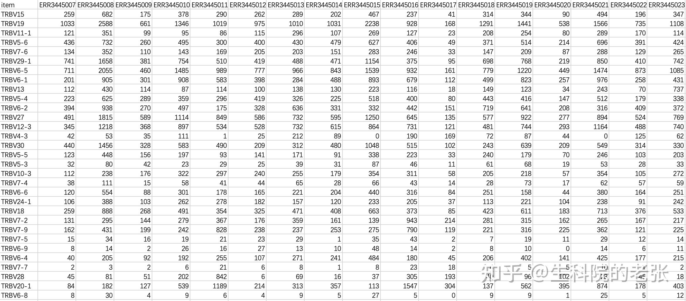
matrix_V.txt
2.15.2 R包DESeq2差异分析:
library(DESeq2)
################################################################################################################################################
input_matrix='/Users/ZYP/Downloads/imm_repertoire/vdjtools_result/matrix_V.txt'#将前面得到的表达信息文件matrix.txt的绝对路径及文件写在此处的''内
input_info='/Users/ZYP/Downloads/imm_repertoire/vdjtools_result/sample_info.txt'#将预先整理的样本信息文件sample_info.txt的绝对路径及文件写在此处的''内
output_file='/Users/ZYP/Downloads/imm_repertoire/vdjtools_result/diffexp_result_V.txt'#将保存输出文件的绝对路径写在此处的''内
label#将样本信息文件sample_info.txt中用于分组进行差异分析的标签名写在此处
batch#将样本信息文件sample_info.txt中用作差异分析因素的标签名写在此处
################################################################################################################################################
input_data <- read.table(input_matrix,header = TRUE,row.names = 1)
input_data <- round(input_data,digits=0)#取整
input_data <- as.matrix(input_data)#转换为矩阵
input_data
info_data <- read.table(input_info,header = TRUE,row.names = 1)
info_data <- as.matrix(info_data)
info_data
dds <- DESeqDataSetFromMatrix(countData = input_data,colData = info_data,design = ~label)#若batch为空则design=~label,否则为design=~batch+label
dds <- DESeq(dds)
result <- results(dds,alpha = 0.1)
summary(result)
result <- result[order(result$padj),]
result_data <- merge(as.data.frame(result),as.data.frame(counts(dds,normalized=TRUE)),by='row.names',sort=FALSE)
names(result_data)[1] <- 'Gene'
write.table(result_data,output_file,sep = '\t',quote=F,row.names = F)输出文件格式如下:
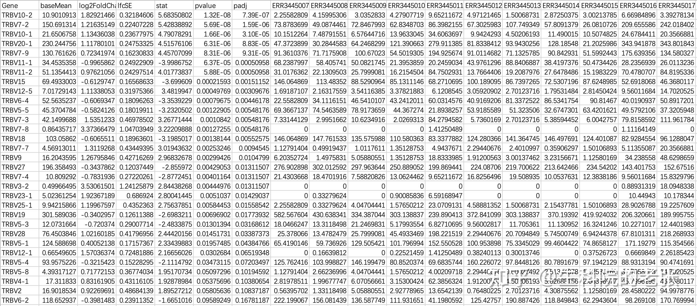
diffexp_result_V.txt
2.15.3 Volcanoplot:
import seaborn as sns, matplotlib.pyplot as plt, pandas as pd, numpy as np
########################################################################################################################
input_file='/Users/ZYP/Downloads/imm_repertoire/vdjtools_result/diffexp_result_J.txt'#请将带有绝对路径的输入文件写在此处的''内
output_file='/Users/ZYP/Downloads/imm_repertoire/vdjtools_result/diffexp_VolcanoPlot_J.pdf'#请将带有绝对路径的输出文件写在此处的''内
########################################################################################################################
list_log2FC=[]
list_padj=[]
index_log2FC=2
index_padj=6
number_row=1
for line in open(input_file):
if number_row==1:
index_log2FC=line[:-1].split('\t').index('log2FoldChange')
index_padj=line[:-1].split('\t').index('padj')
else:
if line.split('\t')[index_log2FC]!='NA' and line.split('\t')[index_padj]!='NA':
list_log2FC.append(float(line.split('\t')[index_log2FC]))
list_padj.append(float(line.split('\t')[index_padj]))
number_row+=1
foldchange=np.asarray(list_log2FC)
pvalue=np.asarray(list_padj)
result = pd.DataFrame({'pvalue': pvalue, 'FoldChange': foldchange})
result['log(pvalue)'] = -np.log10(result['pvalue'])
result['sig'] = 'normal'
result['size'] = np.abs(result['FoldChange']) / 10
result.loc[(result.FoldChange > 1) & (result.pvalue < 0.05), 'sig'] = 'up'
result.loc[(result.FoldChange < -1) & (result.pvalue < 0.05), 'sig'] = 'down'
ax = sns.scatterplot(x="FoldChange", y="log(pvalue)",hue='sig',hue_order = ('up','down','normal'),palette=("#E41A1C","#377EB8","grey"),data=result)
ax.set_ylabel('-log10Padj',fontweight='bold')
ax.set_xlabel('log2FoldChange',fontweight='bold')
ax.spines['top'].set_visible(False)
ax.spines['right'].set_visible(False)
plt.savefig(output_file)
plt.show()结果如下图所示:
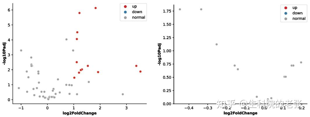
Volcanoplot of V / J genes
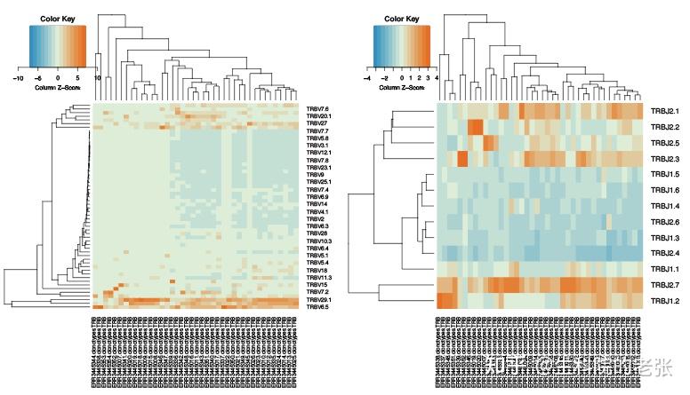
2.15.4 Heatmap:
import seaborn as sns
import pandas as pd
from matplotlib import pyplot as plt
########################################################################################################################
input_file='/Users/ZYP/Downloads/imm_repertoire/vdjtools_result/padj<0.05&log2FC>1or<-1_V.txt'#请将带有绝对路径的输入文件写在此处的''内
output_file='/Users/ZYP/Downloads/imm_repertoire/vdjtools_result/diffexp_heatmap_V.pdf'#请将带有绝对路径的输出文件写在此处的''内
sample_info='/Users/ZYP/Downloads/imm_repertoire/vdjtools_result/sample_info.txt'#请将带有绝对路径的样本分组文件写在此处的''内
########################################################################################################################
list_pos=[]
for line in open(sample_info,'r'):
info=line[:-1].split('\t')
if info[0]!='ID':
if str(info[1])=='Class1':
list_pos.append(info[0])
list_ids=[]
list_samples=[]
list_value_list=[]
list_sample_colors=[]
list_gene_colors=[]
begin_samples=7
index_log2FC=2
index_p=5
number_row=1
for line in open(input_file):
if number_row!=1:
list_ids.append(line[:-1].split('\t')[0])
list_value=[]
for value in line[:-1].split('\t')[begin_samples:]:
list_value.append(float(value))
list_value_list.append(list_value)
log2FC=float(line[:-1].split('\t')[index_log2FC])
p=float(line[:-1].split('\t')[index_p])
if p<0.05 and log2FC>1:
list_gene_colors.append(sns.xkcd_rgb["dark red"])
if p<0.05 and log2FC<-1:
list_gene_colors.append(sns.xkcd_rgb["marine blue"])
else:
begin_samples = line[:-1].split('\t').index('padj') + 1
index_log2FC = line[:-1].split('\t').index('log2FoldChange')
index_padj = line[:-1].split('\t').index('padj')
for sample in line[:-1].split('\t')[begin_samples:]:
list_samples.append(sample)
if sample in list_pos:
list_sample_colors.append(sns.xkcd_rgb["dark red"])
else:
list_sample_colors.append(sns.xkcd_rgb["marine blue"])
number_row+=1
print(len(list_sample_colors))
print(len(list_gene_colors))
data=pd.DataFrame(data=list_value_list,index=list_ids,columns=list_samples)
print(data)
ax=sns.clustermap(data,standard_scale=1,row_colors=list_gene_colors,col_colors=list_sample_colors)
plt.savefig(output_file)
plt.show()结果如下图所示:

Heatmap of diff-expressed V genes (there were no diff-expressed J genes)
<hr/>作者的话:
- 如果你喜欢我的科研创作,欢迎将它分享给更多的研友。一起向着创造和传播知识的目标继续进发吧!
- 学术交流欢迎关注、私信。
原文地址:https://zhuanlan.zhihu.com/p/383280340 |
|

 /3
/3 

 浙公网安备33010802005999号


 2026庆【网站十三周
 2025庆【网站十二周
 2024庆中秋、迎国庆
 2024庆【网站十一周
 2023庆【网站十周年
 2022庆【网站九周年

 发表于 2025-3-12 15:31